Advanced Analytics with Apache Spark: What is Spark?

The challenges of Data Science

The hard truths:

First, the majority of work that goes into conducting successful analyses lie in preprocessing data. Data is messy, and cleansing, munging, fusing, mushing and many other verbs are prerequisites for doing anything useful with it…A typical data (processing) pipeline requires spending far more time in feature engineering and selection than in choosing and writing algorithms. The Data Scientist must choose from a wide variety of potential features (data). Each comes with its own challenges in converting to vectors fit for machine learning algorithms. A system needs to support more flexible transformations than turning a 2-d array (tuple) of doubles into a mathematical model.

Second, iteration. Models typically require multiple passes/scans over the same data to reach convergence. Iteration is also crucial within the Data Scientist’s own workflow, usually the results of a query inform the next query that should run. Feature and algorithm selection, significance testing and finding the right hyper-parameters all require multiple experiments.

Third, implementation. Models need to be operationalised and become part of a production service and may need to be rebuilt periodically or even in real time – analytics in the ‘lab’ vs analytics in the ‘factory’. Exploratory analytics usually occurs in e.g. R, whereas production applications’ data pipelines are written in C++ or Java.

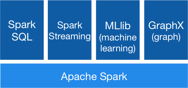
Enter Apache Spark

Apache Spark is an open-source cluster computing framework originally developed in the AMPLab at UC Berkeley. In contrast toHadoop’s two-stage disk-based MapReduce paradigm, Spark’s in-memory primitives provide performance up to 100 times faster for certain applications.^[1] By allowing user programs to load data into a cluster’s memory and query it repeatedly, Spark is well suited to machine learning algorithms.^[2]

Spark is an open-source framework that combines an engine for distributed programs across clusters of machines with an elegant model for writing programs atop it.

Word Count

In this SCALA example, we build a dataset of (String, Int) pairs called counts and then save it to a file:

val file = spark.textFile(“hdfs://…”)
val counts = file.flatMap(line => line.split(” “))
.map(word => (word, 1))
.reduceByKey(_ + _)
counts.saveAsTextFile(“hdfs://…”)

One way to understand Spark is to compare it to its predecessor, MapReduce. Spark maintains MapReduce’s linear scalability and fault tolerance, but extends it in 3 important ways:

First, rather than relying on a rigid map-then-reduce format, Spark’s engine can execture a more general directed acyclic graph (DAG) of operators. 

This means that (rather than MapReduce writing out intermediate results to the distributed filesystem), Spark can pass them directly to the next step in the pipeline.
http://www.dagitty.net/learn/graphs/index.html

Secondly, Spark has a rich set of transformations that enable users to express computation more naturally. Its streamlined API can represent complex pipelines in a few lines of code.

Thirdly, Spark leverages in-memory processing (rather than distributed disk). Developers can materialise any point in a processing pipeline into memory across the cluster, meaning that future steps that want to deal with the same dataset need not recompute it from disk.

Perhaps most importantly, Spark’s collapsing of the full pipeline, from preprocessing to model evaluation, into a single programming environment can dramatically speed up productivity. By packaging an expressive programming model with a set of analytic libraries under REPL it avoids round trips and moving data back and forth. Spark spans the gap between lab and factory analytics, Spark is better at being an operational system than most exploratory systems and better for data exploration that the technologies commonly used in operational systems. Spark also has tremendous versatility offering functionality like SQL, being able to ingest data from streaming services like Flume & Kafka, it has machine learning tools and graph processing capabilities.

MapReduce links

http://wiki.summercode.com/mongodb_aggregation_functions_and_ruby_map_reduce_basics

https://github.com/shimondoodkin/nodejs-mongodb-app/wiki/explanation-of-map-reduce

http://www.mongovue.com/2010/11/03/yet-another-mongodb-map-reduce-tutorial/#comment-117

http://cookbook.mongodb.org/patterns/pivot/

http://stackoverflow.com/questions/9337343/mongodb-map-reduce-tutorial

counting the occurrence of words in a field (column)

How to do it?

I have a series of documents in a MongoDB collection, each doc has 7 columns.

Col7 is a large text field which contains the Ts and Cs, scraped from various websites.

I want to count the freqy of each word in that field, for each object.

So, for example, col 7 in document 1 may contain ‘delete’ 100 times.

Col 7 in doc 90 may contain ‘delete’ 2 times.

More to follow…

================================================================

Thanks to Terradata’s Chris Hillman for the following suggestion:

…That seems like a nice MapReduce task, I’d do it like this

Map

input Key, Value

    <documentID, DocumentText>

Process

    tokenise the document

Output Key, Value

    <documentID concatenated with token, 1> For DocID 50 and token “plum” This would look like 50|plum, 1

Reduce

input Key, Value

    <documentID concatenated with token, 1>

Process

    sum the counts by docid|token

Output Key, Value

    <documentID concatenated with token, count>

Up to you if you use the pipe d”|” delimiter for this or maybe use a tab “\t” to make the output easier to parse I’ve not used     Mongo so I don’t know what format it accepts

For the gold star solution use a “combiner” in the Map step to do a pre-reduce on the docid|token keys and reduce I/O

Basically the same as standard word count but with the docid concatenated on the token

MongoDB’s “Aggregation Framework”

In my earlier post I built up a very simple report using the MongoDB connector in Jaspersoft iReport.

Today I noticed you can natively query MongoDB from within Jaspersoft. See more here

Some examples;

In SQL:

SELECT *
  FROM users
  WHERE age > 25
   AND   age <= 50
  ORDER BY age

When using Mongo:

{
   collectionName : 'users',
   findQuery : { 
        age: { $gt: 25, $lte: 50 } 
   },
   sort : {
        'age': 1
   }
}

See: http://docs.mongodb.org/manual/reference/sql-comparison/

An examples of using MongoDB’s ‘Aggregation Framework‘ which I think as pre-computed views/aggregations/filtered results sets

In SQL:

SELECT cust_id, ord_date, SUM(price) AS total
FROM orders
GROUP BY cust_id, ord_date
HAVING total > 250
ORDER BY total DESC

When using Mongo:

{
   runCommand: {
        aggregate : 'orders',
        pipeline : [
                {
                        $group : {
                                _id : { cust_id: '$cust_id', ord_date: '$ord_date' }
                                total: { $sum : '$price' }
                        }
                },
                { 
                        $match: { 
                                total: { $gt: 250 } } 
                        }
                },
                {
                        $sort : {
                                total : -1
                        }
                }
        ]
}

This got me curious about the aggregation framework. Here’s another couple of examples of how it might be applied.

Each document in this collection has the following form:

{
  "_id": "10280",
  "city": "NEW YORK",
  "state": "NY",
  "pop": 5574,
  "loc": [
    -74.016323,
    40.710537
  ]
}

In these documents:

• The _id field holds the zipcode as a string.
• The city field holds the city.
• The state field holds the two letter state abbreviation.
• The pop field holds the population.
• The loc field holds the location as a latitude longitude pair.

To Calculate States with Populations Over 10 Million

db.zipcodes.aggregate( { $group :
                         { _id : "$state",
                           totalPop : { $sum : "$pop" } } },
                       { $match : {totalPop : { $gte : 10*1000*1000 } } } )

Map/Reduce Queries in MongoDB – for relational dummies (like me!)

Thanks to my ex-colleague and Genius Dina Mohammad for sharing this with me.

QueryMongo.com

And an example of the different query constructs in SQL vs NoSQL worlds, although the example uses Map/Reduce rather than native querying. I know which I prefer!

SELECT person, SUM(score), AVG(score), MIN(score), MAX(score), COUNT(*)
FROM demo
WHERE score > 0 AND person IN (‘bob’,’jake’)
GROUP BY person;

db.demo.group({
“key”: {
“person”: true
},
“initial”: {
“sumscore”: 0,
“sumforaveragescore”: 0,
“countforaveragescore”: 0,
“minscore”: 0,
“maxscore”: 0,
“countstar”: 0
},
“reduce”: function(obj, prev) {
prev.sumscore += obj.score;
prev.sumforaveragescore += obj.score;
prev.countforaveragescore++;
prev.minscore = Math.min(prev.minscore, obj.score);
prev.maxscore = Math.max(prev.maxscore, obj.score);
prev.countstar++;
},
“finalize”: function(prev) {
prev.averagescore = prev.sumforaveragescore / prev.countforaveragescore;
delete prev.sumforaveragescore;
delete prev.countforaveragescore;
},
“cond”: {
“score”: {
“$gt”: 0
},
“person”: {
“$in”: [“bob”, “jake”]
}
}
});